| About Chapter 6 | |
| [Developer] Kai Pan (Ben) Chu Created at: 0000-00-00 00:00 Chp6General | 4 |
| Question / Discussion that is related to Chapter 6 should be placed here | |
4 | |
Easy Difficult Number of votes: 4 | |
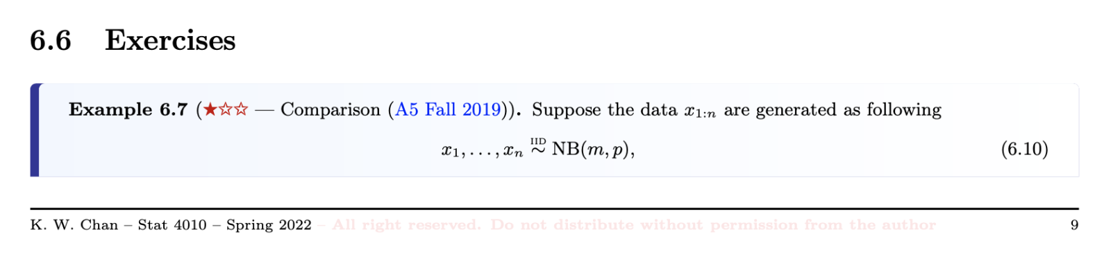
| May I have the answers to ex 6.7 and ex 6.10? | |
| Anonymous Bat Created at: 2022-03-25 18:23 | 1 |
| Will the answer to 2019 fall A5 be released at the website? I hope to check if I solve the exercise correctly. p.s. Ex 6.8 is from the final of 2019 fall, and Ex 6.9 is from the mock final of 2019 fall. | |
| Show 1 reply | |
| [Instructor] Kin Wai (Keith) Chan Created at: 2022-03-26 11:52 | 5 |
| |
| About distribution conditioning on random variables | |
| Anonymous Loris Last Modified: 2022-04-02 16:17 | 3 |
I am confused about the conditional distribution when the condition part are r.v.s. For example, in theorem 6.2, we have $[\theta|x_{1:n}]\approx N(\hat{\theta}_{MLE},\frac{J_*^{-1}}{n})$, the location parameter $\hat{\theta}_{MLE}$ is a r.v. here. So can I say that:
| |
| Show 1 reply | |
| [Instructor] Kin Wai (Keith) Chan Created at: 2022-04-02 12:42 | 6 |
Good questions! Your questions related to the concept of conditional distribution.
| |
| Example 6.10 | |
| Anonymous Lion Created at: 2022-04-04 15:04 | 2 |
For example 6.10, would you be able to tell me the process between these 2 (highlighted) lines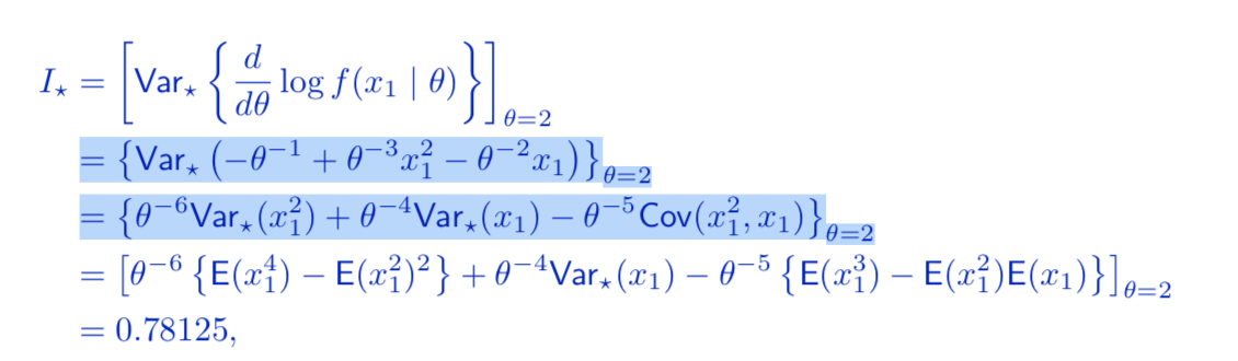 | |
| Show 3 reply | |
| Anonymous Ifrit Created at: 2022-04-04 16:33 | 2 |
| I am confused about these two lines too. I tried to expand the term, but it turns out that an extra 2 appears in the covariance term. Var*( -θ-1 + θ-3 x12 - θ-2 x1 ) = Var*( θ-3 x12 - θ-2 x1 ) = (θ-3)(θ-3)Var*(x12) + 2(θ-3)(-θ-2) Cov*( x12, x1 ) + (-θ-2)(-θ-2)Var*(x1) = θ-6Var*(x12) + θ-4Var*(x1) - 2 θ-5 Cov*( x12, x1 ) | |
| Anonymous Ifrit Created at: 2022-04-04 16:51 | 3 |
| I guess it is a typo maybe… I tried to plug in the values into my derived formula (with an extra 2 in covariance) and I found that the output equals 0.78125, the answer given in the solution. | |
| [TA] Cheuk Hin (Andy) Cheng Created at: 2022-04-04 18:02 | 4 |
| Chi Hei is correct. There should be 2 before the covariance term. Sorry for the typo. | |
| About the model and theta | |
| Anonymous Monkey Created at: 2022-04-08 14:08 | 1 |
| Q1.I want to ask about the difference between f* and theta*, from notes, the f* is true DGP, but we don't know f*, so we use another model to estimate f* and find the parameter for the model we proposed. But since we don't know the true model, how can we measure whether our model is good or not? Q2. Are theta* and theta(MLE) are two for estimating the true parameter for our proposed model? I do not quite understand what's role of theta* in the correctly specified model cases and misspecified model cases. Is that incorrectly specified case, the theta* is equal to the true parameter, and it is different from the true parameter if the model is misspecified? | |
| Show 2 reply | |
| Anonymous Orangutan Last Modified: 2022-04-13 15:10 | 0 |
| sorry, wrong place to post | |
| [TA] Cheuk Hin (Andy) Cheng Created at: 2022-04-11 23:43 | 3 |
| Q1: f* is the true DGP whereas $\theta_*$ is just an unknown quantity related to f*. We are interested in $\theta_*$ because it is the asymptotic mean of the MLE. Let says we want to choose an estimator that has smaller asymptotic variance which is a function of $I_*$ and $J_*$. In practice although we do not know the true DGP, we can still estimate $I_*$ and $J_*$ using our observation. You will see it in part 4. We do not know the true DGP of average temperature. But we can still estimate $I_*$ and $J_*$. The form of $I_*$ and $J_*$ can be derived by our model. The unknown quantity $E_*(\cdot)$ and $Var_*(\cdot)$ for example can be estimated from the data. We may also do simulation to see different estimators perform (in terms of MSE for example) under different pre-determined DGP. For example in this case you may try different mean and variance for f*. Repeat all estimation procedure and compare the performance. Q2: $\theta_*$ is not estimator. It is just an unknown quantity that helps us to describe the asymptotic result of MLE and posterior. For Takumi question, conjugate prior is just an handy tool. Bayesian inference can be performed even we do not have it. In practice, in deed, you may want to consider a model that is easy to work with. But you need to balance the statistical efficiency. | |
| May I ask is the model still useful when the model mis specify the DGP? | |
| Anonymous Mink Created at: 2024-04-05 13:25 | 0 |
| May I ask is the model still useful when the model mis specify the DGP? | |
| Show 1 reply | |
| Anonymous Mink Created at: 2024-04-05 13:29 | 0 |
| I'm also wondering why this chapter is called “Theoretic justification”? Thank you | |
| Example 5.5 | |
| [TA] Di Su Created at: 0000-00-00 00:00 Chp5Eg5 | 0 |
| Example 5.5 (${\color{blue}\star}{\color{blue}\star}{\color{gray}\star}$ Bi-dimensional loss). Usually, aregion estimator \(\widehat{I}\) of\(\theta\) is evaluated according totwo different dimensions: (i) width $\bigstar~$Solution: Denote \(\widehat{I} =[\widehat{L},\widehat{U}]\). The posterior loss is | |
2 | |
Easy Difficult Number of votes: 3 | |
| Posterior Loss | |
| Anonymous Pumpkin Created at: 2024-04-05 10:07 | 0 |
| For the calculation of posterior loss, I understand that $\displaystyle E[\mathbf{1}(\theta\notin \hat{I})|x]=1-\int_{-\infty}^\infty\mathbf{1}(\theta\in\hat{I})\pi(\theta|x)\mathrm{d}\theta=1-\int_{\hat{I}}\pi(\theta|x)\mathrm{d}\theta$ However, I do not understand why $\displaystyle E(k|\hat{I}|\ |x)=k|\hat{U}-\hat{L}|$. Can anyone help me with that? | |
| Show reply | |
| Example 5.3 | |
| [TA] Di Su Created at: 0000-00-00 00:00 Chp5Eg3 | 0 |
| Example 5.3 (${\color{blue}\star}{\color{gray}\star}{\color{gray}\star}$ Transformed parameters). Let\([x_1, \ldots, x_n \mid \theta] \overset{\text{iid}}{\sim} \text{N}(\theta,\sigma^2)\) and
$\bigstar~$Solution:
$\bigstar~$Takeaway: The principle of “equal tails” is invariant, but theprinciple of HPD is not. | |
2 | |
Easy Difficult Number of votes: 3 | |
| Question 2 | |
| Anonymous Pumpkin Created at: 2024-04-04 22:46 | 0 |
| We know from Example 5.2 that $$ \hat{L}_a=\theta_n + z_a\tau_n $$ Let $a = 2.5\%$, $\phi = e^{\hat{L}_a}$, we know that the pdf of $\displaystyle[\phi|x_{1:n}] = \frac{e^{-\frac{(\log\phi -\theta_n)^2}{2\tau_n^2}}}{\sqrt{2\pi\tau_n^2\phi^2}}$, then we have $$ \begin{aligned} \log\phi = \log{ e^{\hat{L}_a}}= \hat{L}_a=\theta_n + z_a\tau_n\\ \log\phi-\theta_n = \theta_n + z_a\tau_n-\theta_n=z_a\tau_n\\ -\frac{(\log\phi -\theta_n)^2}{2\tau_n^2}=-\frac{(z_a\tau_n)^2}{2\tau_n^2}=-\frac{z_a^2}{2}\\ \end{aligned} $$ Therefore, we have $$ \begin{aligned} \pi_\phi(\phi|x_{1:n})= \pi_\phi( e^{\hat{L}_a}|x_{1:n})&=\frac{e^{-\frac{(\log\phi -\theta_n)^2}{2\tau_n^2}}}{\sqrt{2\pi\tau_n^2\phi^2}}\\ &=\frac{e^{-\frac{z_a^2}{2}}}{\sqrt{2\pi}\tau_ne^{\hat{L}_a}}\\ &= \frac{e^{-z_a^2/2}}{e^{\hat{L}_a}\tau_n\sqrt{2\pi}} \end{aligned} $$ My calculation is different from the solution 2, which is $\displaystyle \frac{e^{-1/2}}{e^{\hat{L}_a}\tau_n\sqrt{2\pi}}$, I wonder whether there are some mistakes that I can not arrive the solution. | |
| Show reply | |
| Example 5.2 | |
| [TA] Di Su Created at: 0000-00-00 00:00 Chp5Eg2 | 1 |
| Example 5.2 (${\color{blue}\star}{\color{gray}\star}{\color{gray}\star}$ Normal-Normal model). Let
$\bigstar~$Solution:
$\bigstar~$Takeaway: Credible interval is not confidence interval. | |
3.5 | |
Easy Difficult Number of votes: 2 | |

| Typo | |
| Anonymous Pumpkin Last Modified: 2024-04-04 22:16 | 0 |
| Solution 2. Method 1: By Lemma 5.1 $\textbf{above}$ … | |
| Show reply | |
| About Chapter 5 | |
| [Developer] Kai Pan (Ben) Chu Created at: 0000-00-00 00:00 Chp5General | 2 |
| Question / Discussion that is related to Chapter 5 should be placed here | |
4.7 | |
Easy Difficult Number of votes: 3 | |
| HPD: normalization step | |
| Anonymous Orangutan Last Modified: 2022-03-21 13:26 | 3 |
| I' m still not sure the step of normalization. ①For me, it is weird the sum(d0) and the interval are separated. Is it possible to rewrite like below? ⓶Also, I computed d and I think d is not normalized. Although it is ok to multiply by (theta[2]-theta[1]) again when we compute N,I don't know how to interpret the y axis of posterior distribution(from 0 to 5 in this example). Why we don't use d = d0/sum(d0) , when we plot (theta, d) ? | |
| Show 1 reply | |
| [TA] Di Su Last Modified: 2022-03-23 20:42 | 4 |
| ① It is ok to write like below. ⓶ For a continuous random variable X, it is possible that $f_X(x)>1$, what we want to restrict is $\int_\mathcal{X}f_X(x)\mathrm{d}x\leq1$. We don't use d = d0/sum(d0) when we plot (theta, d) because we want to use Riemman sum, so the term (theta[2]-theta[1]) is needed. | |
| credible interval | |
| Anonymous Mink Created at: 2024-03-29 17:56 | 0 |
| May I ask is there any frequentist's language for the credible interval like confidence interval to reject H0 at confidence... sth like that? | |
| Show reply | |
| Decision Theory | |
| Anonymous Pumpkin Created at: 2024-04-04 22:02 | 0 |
| I wonder why HPD is supported by decision theory while ET is not. Thank you. | |
| Show reply | |
| Example 6.2 | |
| [TA] Di Su Created at: 0000-00-00 00:00 Chp6Eg2 | 3 |
| Example 6.2 (${\color{blue}\star}{\color{blue}\star}{\color{gray}\star}$ Mis-specified model). Let theDGP be \(x_1, \ldots, x_n \overset{\text{iid}}{\sim} \text{Ga}(2)\). Assume a model $\bigstar~$Solution:
$\bigstar~$Intuition: Suppose the prior is \(\theta \sim\text{Ga}(\alpha)/\beta\). The posterior is  $\bigstar~$Experiment: Let \(n = 1000\) sothat the asymptotic arguments apply. In the experiment, we generate\(x_{1:n}\) and then record the valuesof
R code is used. $\bigstar~$Takeaway: If the model is mis-specified,Bayesian and frequentist inference diverge. | |
3.8 | |
Easy Difficult Number of votes: 5 | |
| The divergence between Bayesian and frequentist inference | |
| Anonymous Armadillo Created at: 2024-04-02 18:38 | 1 |
| Considering the divergence between Bayesian and frequentist inference in the case of mis-specified models, what implications does this have for real-world applications where the true underlying distribution might be unknown or misjudged? How can practitioners mitigate the risks of divergent inference in such scenarios, especially when decisions based on these inferences can have significant consequences? Thank you! | |
| Show reply | |
| Example 3.23 | |
| [TA] Chak Ming (Martin), Lee Created at: 0000-00-00 00:00 Chp3Eg23 | 0 |
| Example 3.23 (${\color{blue}\star}{\color{blue}\star}{\color{gray}\star}$ Multivariate normal). Let \([x\mid\theta]\sim \text{N}_p(\theta, I_p)\), where \(\theta = (\theta_1, \ldots, \theta_p)^{\text{T}}\). Prove that if the loss is \(L(\theta, \widehat{\theta}) = \| \theta - \widehat{\theta} \|^2 = \sum_{j=1}^p (\theta_j - \widehat{\theta}_j)^2\), then the minimax estimator of \(\theta\) is \(\widehat{\theta}_{M} = x\). $\bigstar~$Solution:
| |
4 | |
Easy Difficult Number of votes: 1 | |
| Bayes Risk $R(\pi, \hat{\theta}(\sigma))$ | |
| Anonymous Pumpkin Created at: 2024-04-02 13:11 | 0 |
| I tried to use Remark 3.5 to get the Bayes Risk, which is similar to Example 2.2. However, p is not included in the Bayes Risk. So can anyone help me on how to get the Bayes Risk $R(\pi, \hat{\theta}(\sigma))=p\sigma^2/(1+\sigma^2)$? | |
| Show reply | |
| Example 3.22 | |
| [TA] Chak Ming (Martin), Lee Created at: 0000-00-00 00:00 Chp3Eg22 | 0 |
| Example 3.22 (${\color{blue}\star}{\color{gray}\star}{\color{gray}\star}$ Univariate normal). Let \([x_1, \ldots, x_n\mid\theta]\sim \text{N}(\theta, \sigma^2_0)\), where \(\sigma_0^2\) is known. Prove that \(\bar{x}_n\) is minimax under the squared error loss. $\bigstar~$Solution:
| |
5 | |
Easy Difficult Number of votes: 1 | |
| Step 1 | |
| Anonymous Pumpkin Last Modified: 2024-04-01 22:09 | 0 |
| What is the reason behind finding the risk of $a\bar{x}_n+b$? | |
| Show 1 reply | |
| Anonymous Pumpkin Created at: 2024-04-01 22:11 | 0 |
| I see. Since Remark 3.5, $L_2$-risk is $MSE$ | |
| Example 3.16 | |
| [TA] Chak Ming (Martin), Lee Created at: 0000-00-00 00:00 Chp3Eg16 | 0 |
| Example 3.16 (${\color{blue}\star}{\color{blue}\star}{\color{gray}\star}$ Computation of Bayes estimators). Let \([x_1, \ldots, x_n \mid \theta] \overset{ \text{iid}}{\sim} \text{Unif}[0,\theta]\) and \(\theta \sim \beta/\text{Ga}(\alpha)\). Write \(x_{(n)} = \max(x_{1:n})\). Prove that the Bayes estimator under \(\mathcal{L}^2\)-loss is \[\begin{align}\label{eqt:BeyesUnif_form1} \widehat{\theta} = \frac{I_0}{I_1}, \qquad \text{where}\qquad I_k = \int_{x_{(n)}}^{\infty}\frac{e^{-\beta/\theta}}{\theta^{n+\alpha+k}} \, \text{d}\theta. \tag{3.2} \end{align}\] Prove that, for \(k\geq 0\), \[I_k = \frac{\Gamma(n+\alpha+k-1)}{\beta^{n+\alpha+k-1}} \times \texttt{pchisq}\left(\frac{2\beta}{x_{(n)}};2(n+\alpha+k-1) \right),\] where \(\texttt{pchisq}(\cdot; k)\) is the CDF of \(\chi^2_k\). Hence, \[\begin{align}\label{eqt:BeyesUnif_form2} \widehat{\theta} = \frac{\beta}{n+\alpha-1}\frac{\texttt{pchisq}\left({2\beta}/{x_{(n)}};2(n+\alpha-1) \right)}{\texttt{pchisq}\left({2\beta}/{x_{(n)}};2(n+\alpha) \right)} \tag{3.3} \end{align}\] Discuss which form ((\ref{eqt:BeyesUnif_form1}) or (\ref{eqt:BeyesUnif_form2})) of the Bayes estimator \(\widehat{\theta}\) do you prefer in practice. $\bigstar~$Solution: Note that \(\theta\sim\beta/\text{Ga}(\alpha)\) means that \(\theta\) follows an inverse-Gamma distribution with shape and scale parameters \(\alpha,\beta\). Upon checking, we know that \(f(\theta) \propto \theta^{-\alpha-1} e^{-\beta/\theta}\). Then the posterior of \(\theta\) is \[\begin{align} f(\theta\mid x_{1:n}) &\propto& f(\theta)\prod_{i=1}^n f(x_i \mid \theta) \\ &\propto& \theta^{-\alpha-1} e^{-\beta/\theta} \prod_{i=1}^n \left\{ \frac{1}{\theta} \mathbb{1}(x_{(n)}\leq \theta) \right\} \\ &=& \frac{1}{\theta^{\alpha+1+n}} e^{-\beta/\theta} \mathbb{1}(x_{(n)}\leq \theta) =: g(\theta), \end{align}\] i.e., \(f(\theta\mid x_{1:n}) = {g(\theta)}/{C}\), where \(C = \int_{0}^{\infty} g(\theta)\, \text{d}\theta\). By Theorem 3.2(1), the Bayes estimator is \[\begin{align} \widehat{\theta} = \frac{\int_{0}^{\infty} \theta g(\theta)\, \text{d}\theta}{\int_{0}^{\infty} g(\theta)\, \text{d}\theta} =\frac{I_0}{I_1}. \end{align}\] Let \(t = 2\beta/\theta\). Changing the variable in the integral \(I_k\), we have \[\begin{align} I_k &=& \int_{0}^{2\beta/x_{(n)}} \frac{e^{-t/2} }{(2\beta/t)^{n+\alpha+k}} 2\beta t^{-2}\, \text{d}t \quad = \quad \int_{0}^{2\beta/x_{(n)}} \frac{e^{-t/2} t^{n+\alpha+k-2}}{(2\beta)^{n+\alpha+k-1}} \, \text{d}t \\ &=&\frac{1}{\beta^{h/2}}\int_{0}^{2\beta/x_{(n)}} \frac{e^{-t/2} t^{h/2-1}}{2^{h/2}}\, \text{d}t \quad= \quad \frac{\Gamma(h/2)}{\beta^{h/2}} \times \texttt{pchisq}\left(\frac{2\beta}{x_{(n)}};h \right), \end{align}\] where \(h = 2(n+\alpha+k-1)\), and the last line is obtained by matching the density of \(\chi_h^2\). Form (\ref{eqt:BeyesUnif_form2}) is preferred because of the following reasons. Form (\ref{eqt:BeyesUnif_form1}) requires compute two integrals, which do not have a close form solution. Computing them in practice requires numerical techniques. It is not difficult but still requires some effort. Form (\ref{eqt:BeyesUnif_form2}) can be easily computed by most statistical software because the integrals have been rewritten as the CDF of some \(\chi^2\) random variables. $\bigstar~$Experiment: Suppose the DGP is \(x_{1:n}\sim \text{Unif}[0,\theta^{\star}]\) with true value \(\theta^{\star} = 3\). The log of squared-bias, variance and MSE of the MLE \(\widehat{\theta}_{MLE} = \max(x_{1:n})\) and the Bayes estimator \(\widehat{\theta}\) are computed for \(n = 1,2,\ldots, 30\). .png) In terms of MSE, the Bayes estimator is more attractive than the MLE for both small and large \(n\). Can you think of any other estimator of \(\theta\) that has a similar performance as the Bayes estimator? | |
4 | |
Easy Difficult Number of votes: 1 | |
| Experiment | |
| Anonymous Pumpkin Last Modified: 2024-04-01 20:43 | 0 |
| |
| Show reply | |
| Exercise 4.2 | |
| [TA] Chak Ming (Martin), Lee Last Modified: 2024-03-23 10:41 A4Ex4.2 | 4 |
| " Related last year's exercise and discussion can be found here. Exercise 2 (Horse racing (40%)). Hong Kong Jocemph Club (HKJC) organizes approximately 700 horse races every year. This exercise analyses the effect of draw on winning probability. According to HKJC: The draw refers to a horse’s position in the starting gate. Generally speaking, the smaller the draw number, the closer the runner is to the insider rail, hence a shorter distance to be covered at the turns and has a slight advantage over horses with bigger draw numbers. The dataset horseRacing.txt, which is a modified version of the dataset in the GitHub project HK-Horse-Racing, can be downloaded from the course website. It contains all races from 15 Sep 2008 to 14 July 2010. There are six columns:race (integral): race index (from 1 to 1364).distance (numeric): race distance per meter (1000, 1200, 1400, 1600, 1650, 1800, 2000, 2200, 2400).racecourse (character): racecourse (""ST"" for Shatin, ""HV"" for Happy Valley).runway (character): type of runway (""AW"" for all weather track, ""TF"" for turf).draw (integral): draw number (from 1 to 14).position (integral): finishing position (from 1 to 14), i.e., position=1 denotes the first one who completed the race.The first few lines of the dataset are shown below. Rcodetag2 In this example, we consider all races that (i) took placed in the turf runway of the Shatin racecourse, (ii) were of distance 1000m, 1200m, 1400m, 1600m, 1800m and 2000m; and (iii) used draws 1–14. Let \(n\) be the total number of races satisfying the above conditions; \(\texttt{position}_{ij}\) be the position of the horse that used the \(j\)th draw in the \(i\)th race for each \(i,j\). For each \(i=1, \ldots, n\), denote \[x_i = \mathbb{1}\bigg( \frac{1}{|\texttt{draw}_i\cap[1,7]|}\sum_{j\in\texttt{draw}_i\cap[1,7]} \texttt{position}_{ij} < \frac{1}{|\texttt{draw}_i\cap[8,14]|}\sum_{j\in\texttt{draw}_i\cap[8,14]} \texttt{position}_{ij} \bigg),\] Denote the entire dataset by \(D\) for simplicity. Suppose that \[\begin{aligned} \left[x_i \mid \theta_{\texttt{distance}_i} \right] & \overset{ {\perp\!\!\!\!\perp } }{\sim} & \text{Bern}(\theta_{\texttt{distance}_i}), \qquad i=1,\ldots,n\label{eqt:raceModel1}\\ \theta_{1000},\theta_{1200},\theta_{1400},\theta_{1600},\theta_{1800},\theta_{2000} & \overset{ \text{iid}}{\sim} & \pi(\theta),\label{eqt:raceModel2}\end{aligned}\] where \(\pi(\theta) \propto \theta^2(1-\theta^2)\mathbb{1}(0<\theta<1)\) is the prior density. (10%) What are the meanings of the \(x\)’s and \(\theta\)’s? (10%) Test \(H_0: \theta_{1000}\leq 0.5\) against \(H_0: \theta_{1000}> 0.5\). (10%) Compute 95% credible interval for each \(\theta_{1000},\theta_{1200},\ldots,\theta_{2000}\). Plot them on the same graph. (10%) Interpret your results in part (3). Use no more than about 100 words. " | |
4.5 | |
Easy Difficult Number of votes: 11 | |
| small typo "H1" in Ex4.2 | |
| Anonymous Mink Created at: 2024-03-29 12:06 | 1 |
.png) | |
| Show reply | |
Apply tag, filter or search to load more result